The Trespasser Bumpmap Format

Introduction

There is a group us trying to create a level editor for the game Trespasser. One thing we had to do was figure out the format of the bump-mapped textures. This page gives an introduction to bumpmapping, and describes my efforts to decode Trespasser bump-mapped textures. (If I'm mixing up my terms, check out the definitions I've tried to stick to, listed at the bottom of the page)

Introduction to Bumpmapping

When a polygon is rendered, one has to compute how bright to render it.

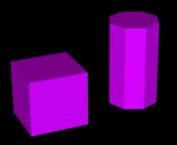
The most simple way to shade a polygon is to calculate the angle between the polygon normal and the incoming light source, and apply some function to the angle to get the intensity. Then the polygon is shaded with a flat colour corresponding to that intensity. This works fine for objects made of flat surfaces, like cubes.
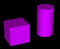
If we are tring to represent a curved surface with the above method, it will look chunky. An improvement is to calculate the normals at the edges, and interpolate between them in the middle of the polygon. This allows the intensity to change accross the polygon, and gives a smoother finish.
If the surface is not smooth, it will requires many more polygons to represent it. This however is not possible given the limitations of real-time rendering. One alternative is to use bumpmapping. This technique modifies the directions of the normals on a large flat polygon, to simulate a surface that is not actually flat.

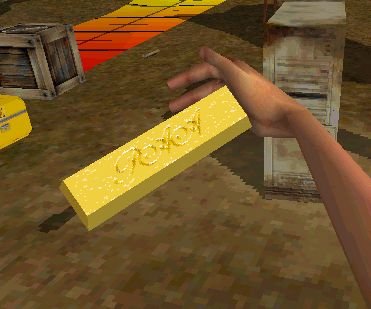
Here is an example of a bump-mapped gold bar in Trespasser. Note that although the top surface of the bar is rendered as one flat polygon, the surface does not catch the light all at once, giving the appearance of a rough surface with indented writing. (click for a bigger picture)

Reverse-engineering the Trespasser bumpmap files

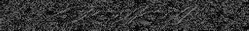
The bump-mapped textures are stored as 16bits per texel. We had already worked out that the high 6 bits store the colour data, and are an index into a palette. If we extract that portion of the data we get:

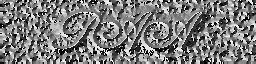
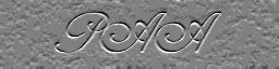
This leaves 10 bits for the bumpmap data. If we view that data as a greyscale image it looks like this: (remembering that 10 bits won't fit into a single 8 bit pixel, thus every second pixel represents just 2 bits of the bumpmap data)

The most user-friendly way to store the data for bump-mapping is as a height-field ('heightmap'). But the previous image does not look like nice slowly changing height values!

My next thought was that the height-field would be stored as the x and y components of the surface normal. I would have stored x and y components of the normal as 5 bits each. Because they would be the derivatives of a smooth height-field, if we viewed the components as greyscale they should look similar.

To test this I broke each texel up into two parts each of 5 bits. It did not look right though. So I tried breaking it into uneven parts, and look what popped out of the lower 4 bits:

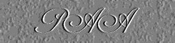
and for the high 6 bits:

But these don't seem like they are the x and y components of the normal, because they don't look alike, and the data is not broken evenly as 5 bits each.

Concentrating on the first image of the lower 4 bits, if we assume that the original height-field is of depressed (or raised) writing, then this image gets darker at the edges of the depression. So it looks like a measure of the 'steepness' of the height-field (H_v the vertical component of height-field normal).

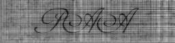
Next we have a close up of the image of the high 6 bits:

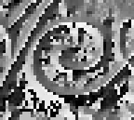There seems to be a smooth change in the data values as we trace around the spiral. It looks rather like it's measuring the angle from the centre of the spiral. Which could certainly be measuring which horizontal direction the height-field normal is facing (H_h the horizontal component of height-field normal).

Great, we now have a value measuring the steepness of the height-field, and another measuring the horizontal direction of the normal. But what I really want is the original height-field. So some calculus formulas pop into mind.

    angle = tan^-1(y/x),  radius = sqrt(x²+y²)

The horizontal component H_h was fairly certainly measured the horizontal angle of the normal vector from some reference point. However I could not tell whether the vertical component H_v was the vertical angle of the normal vector, or the z-component of the normal vector (=cos(angle). In the first case we have:

    n_x = cos(H_h)*H_v  and n_y = sin(H_h)*H_v

and in the second.

    n_x = cos(H_h)*cos(H_v)  and n_y = sin(H_h)*cos(H_v)

I chose the first because it looked nicer. [I later found out that it was actually the second method! I have not reworked the below]

Lets apply the formulas to calculate the x and y components of the normal.

These now look like the 'emboss' option available in many 2d graphics programs. They hopefully represent the partial derivatives of the height-field we are trying to find (partial derivatives = directional derivatives in the horizontal and vertical directions).

Now comes the tricky part. Given the two partial derivatives of our heightfield, we want to compute the original height values. And to make things worse the derivatives are discrete.

Let's do a simple 1D Euler integration, scanning horizontally, and another vertically. However we have a problem. To generate the original function given it's derivatives, one must know the initial conditions ie. the actual values of the height-field along the edges in our case. But we don't know them. Oh well, lets integrate anyway assuming the edges are level at half height:

Integrating left to right: 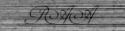and bottom to top:

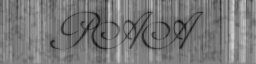
The original height-field is beginning to emerge, and it looks like the writing is depressed (darker colours represent lower heights). One can see the streaks caused by the fact that we are integrating each line separately. This is compounded by the discrete nature of the data, and the inaccurate Euler integration. The effects of the unknown initial conditions are subtly apparent as a slight lack of contrast or 'flatness' near one edge of each image.

A poorman's fix would be to take the average of these two heightmaps:

That's an improvement. But better would be to average the values obtained by the two integration directions as we compute them in the first place. In this way each integration line is using knowledge of it's neighbours to reduce the errors..

Wow, that's much better. However the diagonal streaks are still artifacts. I tested that by doing the integration top-down, and the diagonals changed direction.

The future

Things I want to try next:

Use a better integration method. Each streak seems to go off erroneously in one direction (higher or lower) and stay there. This suggests that the height was consistently being over or under estimated, and is a classic symptom of the Euler method. The Midpoint method should greatly reduce this artifact.
Estimate the initial conditions. I'm currently assuming the edges of the height-field are level at half height. A better way is to assume the height only at one point, say the bottom left corner. Then do a one-dimensional integration horizontally to get the initial conditions for the bottom edge. Similarly a vertical integration to get the ICs for the left edge. Then proceed with the 2-d integration as before. Thus we are left with only one unknown point.

Application to Trespasser

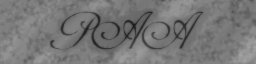
Let's see if what we've learnt works. First we create some of our own colour and height maps:

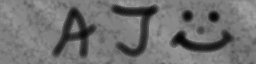
Then do the reverse of the above process. First generating the directional derivatives:

converting to polar coordinates

and insert them into the Trespasser data files. Finally, we run the game:

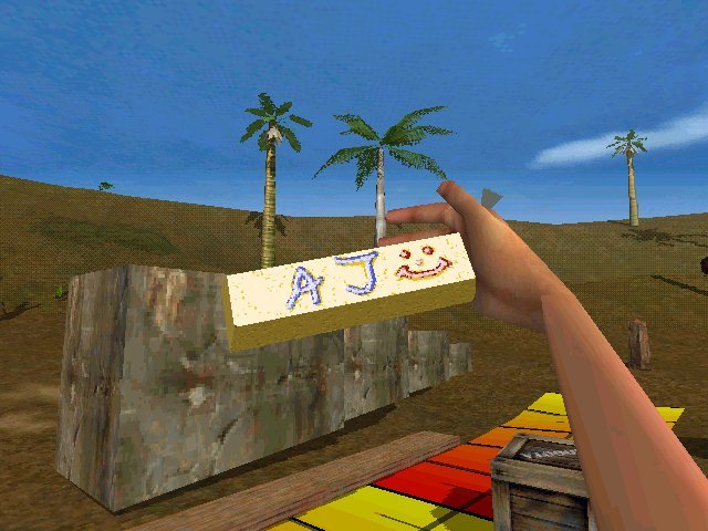
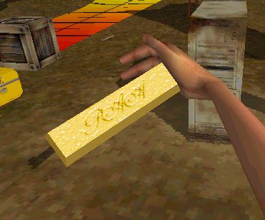
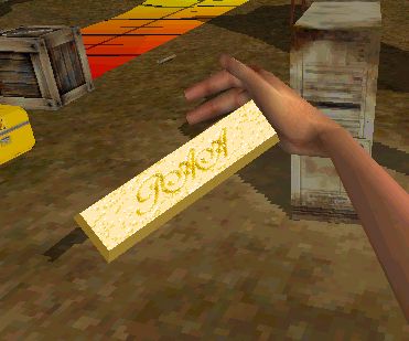
Behold, we have a nice, personalised, bump-mapped gold bar!

Terms

Heightmap/height-field	Rectangular grid of points representing a smooth surface. Higher values are represented as white when displayed as an image
Bumpmap	The heightmap when converted to the form that Trespasser uses
Bumpmapping	The process of rendering a surface while nudging the normal slightly to give the impression that the surface is not smooth, but has detail.